5. Report and make reproducible

The last step is writing it up so a reader can evaluate your analysis and a replicator can rerun it.

Methods section

A complete methods section covers the corpus, the preprocessing, the model and K, the covariate specification, and the validation. A template:

We used [LDA / STM / …] to identify latent topics in a corpus of N documents drawn from [population], covering [time span]. The unit of analysis is the [article / paragraph / speech]; long documents were segmented into chunks of ≤ W words. After preprocessing (lowercasing, removing punctuation and a [SMART + custom] stopword list, pruning terms in fewer than a documents or more than b% of documents, and detecting collocations), the vocabulary contained M terms and T tokens.

We estimated models with K = [value] topics. [Rationale: theory + a searchK scan over K ∈ {…}, balancing semantic coherence, exclusivity, and interpretability; results were robust to K ∈ {…}.] For the STM, topic prevalence was modeled as a function of [covariates]. We fixed the random seed (seed = …) for reproducibility.

We validated the topics with word- and document-intrusion tests ([accuracy / agreement]), per-topic coherence and exclusivity, and bootstrap stability across B resamples; [k] topics flagged as unstable are interpreted cautiously. Software: topica [version].

Results section

• A topic table: each topic's label, its top probability and FREX words, and its overall prevalence.
• Covariate effects with (clustered) standard errors and intervals.
• Representative quotes for the topics you interpret: close reading, not just word lists.

import pandas as pd
import topica

labels = topica.label_topics(model.topic_word, model.vocabulary, n=7)
prevalence = model.doc_topic.mean(axis=0)
table = pd.DataFrame({
    "topic": range(model.num_topics),
    "prevalence": prevalence,
    "top_words_frex": [", ".join(w for w, _ in labels[t]["frex"])
                       for t in range(model.num_topics)],
})
table.to_csv("topic_table.csv", index=False)

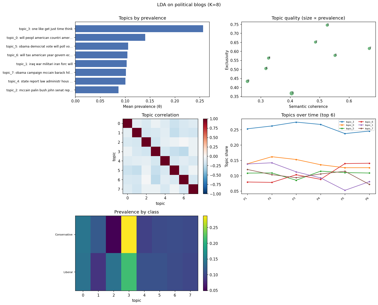
For an at-a-glance figure of the whole model, topica.plot_report composes the diagnostics into one matplotlib Figure you can save straight to a publication or supplement. Panels are adaptive: topic prevalence (with each topic's top words) and the coherence-vs-exclusivity quality plot are always drawn, and the topic-correlation heatmap, topics over time, and prevalence by class appear when you pass texts, timestamps, or groups.

fig = topica.plot_report(model, texts=texts, timestamps=year, groups=party)
fig.savefig("model_report.png", dpi=200)   # or .pdf

The example above is reproducible with python examples/plot_report_example.py.

Supplementary materials

Put in the appendix / replication archive:

• The full topic–word distributions and the document–topic matrix.
• Robustness to K (the headline result at neighboring K).
• Preprocessing details and the exact stopword list.
• Validation results (intrusion accuracy, coherence/exclusivity per topic, stability scores).

import numpy as np
np.savetxt("phi.csv", model.topic_word, delimiter=",")   # topics × words
np.savetxt("theta.csv", model.doc_topic, delimiter=",")  # docs × topics
model.save("model.tt")                                    # full state, reloadable

Make the pipeline reproducible

• Fix every seed. topica fits are bit-for-bit deterministic for a given seed, across machines and core counts. State the seeds you used.
• Script the whole pipeline end to end, from raw text → preprocessing → fit → tables/figures, so it runs from one command.
• Pin versions. Record the topica and NumPy versions (topica.__version__).
• Share the model. model.save(path) writes the complete fitted state; Model.load(path) brings it back, so reviewers can reproduce every number without refitting.

You're done

A corpus you can defend, a K you can justify, topics you've validated, effects with honest uncertainty, and a pipeline anyone can rerun. That is a topic-modeling analysis a social-science journal can publish.

See the worked examples for this workflow applied end to end on real data.